Multivariate stable distribution

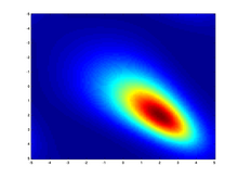
The multivariate stable distribution is a multivariate probability distribution that is a multivariate generalisation of the univariate stable distribution. The multivariate stable distribution defines linear relations between stable distribution marginals. In the same way as for the univariate case, the distribution is defined in terms of its characteristic function.

multivariate stable

Probability density function Heatmap showing a Multivariate (bivariate) stable distribution with α = 1.1
Parameters	$\alpha \in (0,2]$ — exponent $\delta \in \mathbb {R} ^{d}$ - shift/location vector $\Lambda (s)$ - a spectral finite measure on the sphere
Support	$u\in \mathbb {R} ^{d}$
PDF	(no analytic expression)
CDF	(no analytic expression)
Variance	Infinite when $\alpha <2$
CF	see text

The multivariate stable distribution can also be thought as an extension of the multivariate normal distribution. It has parameter, α, which is defined over the range 0 < α ≤ 2, and where the case α = 2 is equivalent to the multivariate normal distribution. It has an additional skew parameter that allows for non-symmetric distributions, where the multivariate normal distribution is symmetric.

Definition

Let $\mathbb {S}$ be the unit sphere in $\mathbb {R} ^{d}\colon \mathbb {S} =\{u\in \mathbb {R} ^{d}\colon |u|=1\}$. A random vector, $X$, has a multivariate stable distribution - denoted as $X\sim S(\alpha ,\Lambda ,\delta )$ -, if the joint characteristic function of $X$ is

$\operatorname {E} \exp(iu^{T}X)=\exp \left\{-\int \limits _{s\in \mathbb {S} }\left\{|u^{T}s|^{\alpha }+i\nu (u^{T}s,\alpha )\right\}\,\Lambda (ds)+iu^{T}\delta \right\}$

where 0 < α < 2, and for $y\in \mathbb {R}$

$\nu (y,\alpha )={\begin{cases}-\mathbf {sign} (y)\tan(\pi \alpha /2)|y|^{\alpha }&\alpha \neq 1,\\(2/\pi )y\ln |y|&\alpha =1.\end{cases}}$

This is essentially the result of Feldheim, that any stable random vector can be characterized by a spectral measure $\Lambda$ (a finite measure on $\mathbb {S}$) and a shift vector $\delta \in \mathbb {R} ^{d}$.

Parametrization using projections

Another way to describe a stable random vector is in terms of projections. For any vector $u$, the projection $u^{T}X$ is univariate $\alpha -$stable with some skewness $\beta (u)$, scale $\gamma (u)$ and some shift $\delta (u)$. The notation $X\sim S(\alpha ,\beta (\cdot ),\gamma (\cdot ),\delta (\cdot ))$ is used if X is stable with $u^{T}X\sim s(\alpha ,\beta (\cdot ),\gamma (\cdot ),\delta (\cdot ))$ for every $u\in \mathbb {R} ^{d}$. This is called the projection parameterization.

The spectral measure determines the projection parameter functions by:

$\gamma (u)={\Bigl (}\int _{s\in \mathbb {S} }|u^{T}s|^{\alpha }\Lambda (ds){\Bigr )}^{1/\alpha }$

$\beta (u)=\int _{s\in \mathbb {S} }|u^{T}s|^{\alpha }\mathbf {sign} (u^{T}s)\Lambda (ds)/\gamma (u)^{\alpha }$

$\delta (u)={\begin{cases}u^{T}\delta &\alpha \neq 1\\u^{T}\delta -\int _{s\in \mathbb {S} }{\tfrac {\pi }{2}}u^{T}s\ln |u^{T}s|\Lambda (ds)&\alpha =1\end{cases}}$

Special cases

There are special cases where the multivariate characteristic function takes a simpler form. Define the characteristic function of a stable marginal as

$\omega (y|\alpha ,\beta )={\begin{cases}|y|^{\alpha }\left[1-i\beta (\tan {\tfrac {\pi \alpha }{2}})\mathbf {sign} (y)\right]&\alpha \neq 1\\|y|\left[1+i\beta {\tfrac {2}{\pi }}\mathbf {sign} (y)\ln |y|\right]&\alpha =1\end{cases}}$

Isotropic multivariate stable distribution

The characteristic function is $E\exp(iu^{T}X)=\exp\{-\gamma _{0}^{\alpha }|u|^{\alpha }+iu^{T}\delta )\}$ The spectral measure is continuous and uniform, leading to radial/isotropic symmetry. For the multinormal case $\alpha =2$, this corresponds to independent components, but so is not the case when $\alpha <2$. Isotropy is a special case of ellipticity (see the next paragraph) – just take $\Sigma$ to be a multiple of the identity matrix.

Elliptically contoured multivariate stable distribution

The elliptically contoured multivariate stable distribution is a special symmetric case of the multivariate stable distribution. If X is α-stable and elliptically contoured, then it has joint characteristic function $E\exp(iu^{T}X)=\exp\{-(u^{T}\Sigma u)^{\alpha /2}+iu^{T}\delta )\}$ for some shift vector $\delta \in R^{d}$ (equal to the mean when it exists) and some positive definite matrix $\Sigma$ (akin to a correlation matrix, although the usual definition of correlation fails to be meaningful). Note the relation to characteristic function of the multivariate normal distribution: $E\exp(iu^{T}X)=\exp\{-(u^{T}\Sigma u)+iu^{T}\delta )\}$ obtained when α = 2.

Independent components

The marginals are independent with $X_{j}\sim S(\alpha ,\beta _{j},\gamma _{j},\delta _{j})$, then the characteristic function is

$E\exp(iu^{T}X)=\exp \left\{-\sum _{j=1}^{m}\omega (u_{j}|\alpha ,\beta _{j})\gamma _{j}^{\alpha }+iu^{T}\delta )\right\}$

Observe that when α = 2 this reduces again to the multivariate normal; note that the iid case and the isotropic case do not coincide when α < 2. Independent components is a special case of discrete spectral measure (see next paragraph), with the spectral measure supported by the standard unit vectors.

Heatmap showing a multivariate (bivariate) independent stable distribution with α = 1

Heatmap showing a multivariate (bivariate) independent stable distribution with α = 2

Discrete

If the spectral measure is discrete with mass $\lambda _{j}$ at $s_{j}\in \mathbb {S} ,j=1,\ldots ,m$ the characteristic function is

$E\exp(iu^{T}X)=\exp \left\{-\sum _{j=1}^{m}\omega (u^{T}s_{j}|\alpha ,1)\lambda _{j}^{\alpha }+iu^{T}\delta )\right\}$

Linear properties

If $X\sim S(\alpha ,\beta (\cdot ),\gamma (\cdot ),\delta (\cdot ))$ is d-dimensional, A is an m x d matrix, and $b\in \mathbb {R} ^{m},$ then AX + b is m-dimensional $\alpha$-stable with scale function $\gamma (A^{T}\cdot ),$ skewness function $\beta (A^{T}\cdot ),$ and location function $\delta (A^{T}\cdot )+b^{T}.$

Inference in the independent component model

Recently it was shown how to compute inference in closed-form in a linear model (or equivalently a factor analysis model), involving independent component models.

More specifically, let $X_{i}\sim S(\alpha ,\beta _{x_{i}},\gamma _{x_{i}},\delta _{x_{i}}),i=1,\ldots ,n$ be a set of i.i.d. unobserved univariate drawn from a stable distribution. Given a known linear relation matrix A of size $n\times n$, the observation $Y_{i}=\sum _{i=1}^{n}A_{ij}X_{j}$ are assumed to be distributed as a convolution of the hidden factors $X_{i}$. $Y_{i}=S(\alpha ,\beta _{y_{i}},\gamma _{y_{i}},\delta _{y_{i}})$. The inference task is to compute the most probable $X_{i}$, given the linear relation matrix A and the observations $Y_{i}$. This task can be computed in closed-form in O(n³).

An application for this construction is multiuser detection with stable, non-Gaussian noise.

See also

• Multivariate Cauchy distribution
• Multivariate normal distribution

Resources

• Mark Veillette's stable distribution matlab package http://www.mathworks.com/matlabcentral/fileexchange/37514
• The plots in this page where plotted using Danny Bickson's inference in linear-stable model Matlab package: https://www.cs.cmu.edu/~bickson/stable