
Original file (1,600 × 3,200 pixels, file size: 1.66 MB, MIME type: image/png)
| This is a file from the Wikimedia Commons. Information from its description page there is shown below. Commons is a freely licensed media file repository. You can help. |
Summary
| Description |
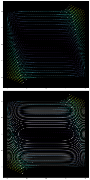
English: A vector field in the plane. The function satisfies , which satisfies the LaSalle's invariance principle, showing that the origin is asymptotically stable.
Plotted in Julia by the following code. ```julia using CairoMakie, LinearAlgebra
df(x, y) = [-y - x^3; x^5] lyapf(x, y) = x^6 + 3y^2 using Interact
scene = Figure(resolution = (1600, 3200)) Axis(scene[1,1], backgroundcolor = "black")
xmin, xmax, xres = -1, 1, 41 ymin, ymax, yres = -1, 1, 41 x = range(xmin, stop = xmax, length = xres) y = range(ymin, stop = ymax, length = yres) xs = repeat(x, outer=length(y)) ys = repeat(y, inner=length(x))
vectors = df.(xs, ys) us = map((x) -> x[1], vectors) vs = map((x) -> x[2], vectors) us /= 5 vs /= 5 n = vec(norm.(vectors)) n /= maximum(n) / 10 arrows!(xs, ys, us, vs, arrowsize = n, linecolor=n, arrowcolor = :white) Axis(scene[2,1], backgroundcolor = "black")
arrows!(xs, ys, us, vs, arrowsize = n, linecolor=n, arrowcolor = :white)
zs = lyapf.(xs, ys) Makie.contour!(xs, ys, zs, levels = 30, linewidth = 2, colormap = :grayC)
save("LaSalle.png", scene) ``` |
| Date | |
| Source | Own work |
| Author | Cosmia Nebula |


Licensing
- You are free:
- to share – to copy, distribute and transmit the work
- to remix – to adapt the work
- Under the following conditions:
- attribution – You must give appropriate credit, provide a link to the license, and indicate if changes were made. You may do so in any reasonable manner, but not in any way that suggests the licensor endorses you or your use.
- share alike – If you remix, transform, or build upon the material, you must distribute your contributions under the same or compatible license as the original.
File history
Click on a date/time to view the file as it appeared at that time.
| Date/Time | Thumbnail | Dimensions | User | Comment | |
|---|---|---|---|---|---|
| current | 07:03, 28 June 2022 | | 1,600 × 3,200 (1.66 MB) | Cosmia Nebula | Uploaded while editing "LaSalle's invariance principle" on en.wiki.x.io |